tl;dr Someone asked me to make a surface mesh of a lizard brain, so I did. Skip to the third section to see how. It can be downloaded here.
I recently received the following:
Dear Daniel Hoops,
I hope this email finds you well.
My name is [redacted], and I am part of the [redacted] team. It is a pleasure to reach out to you.
We are currently working on an exhibition project [for redacted art project], and one of the topics we are exploring is brain morphology. In this regard, we would like to include various replicas of animal brains to help illustrate this subject, one of which is the lizard brain.
While reviewing scientific studies that used CT or MRI to examine lizard brains, we came across the following paper:
Hoops D, Weng H, Shahid A, Skorzewski P, Janke AL, Lerch JP, Sled JG. A fully segmented 3D anatomical atlas of a lizard brain. Brain Struct Funct. 2021 Jul;226(6):1727-1741. doi: 10.1007/s00429-021-02282-z. Epub 2021 Apr 30. PMID: 33929568.
Since you are listed as the corresponding author, we wanted to reach out to kindly ask whether it might be possible for you to share the 3D images of the lizard brain with us, or if there is another institution or researcher we should contact regarding this request.
Additionally, we are also looking to include replicas of other animal brains, such as whale, wolf and crow. If you have any information or studies related to these species, we would truly appreciate any guidance or recommendations you could provide.
Thank you very much for your time and consideration. We would be grateful for any assistance or advice you can offer.
After some back and forth to figure out what exactly they were looking for, I finally was able to reply substantively:
Hi [redacted],
I have included below a link to download a surface mesh file (.stl) of the brain of a lizard called the Swift Dragon (Ctenophorus modesta). When I published the paper on this brain it was called the Tawny Dragon (Ctenophorus decresii) but it has since been changed. Is this the sort of thing you were looking for?
The volume of this brain is 0.107 ml and the weight of the brain is 0.11 g.
It may be interesting for you to note that the olfactory bulbs are not included here. That's because they are on long stalks and are located far away from the rest of the brain. Please let me know if this is a problem and I can try to generate something for you that includes the olfactory bulbs, but it won't be as pretty as what I've sent you here.
Have you had any luck with the other brains you were looking for?
How I made the surface mesh:
Because it was an interesting process that I’d never had to do before, I thought I’d include here how I made a surface mesh from the 3D MRI-based model of a lizard brain that I’d published. The model itself can be downloaded from the Open Science Framework page associated with this paper. The file name is “CdecresiiModel.nii”.
The software I use to manipulate MRI images is called the minc toolkit, and I often struggle because I am not someone who programs or uses command-line software outside of R and minc. Anyone more familiar with programming and command line computing will recognize that what I’m presenting is quite basic. Nonetheless, I hope somebody out there finds it helpful and, if you are someone who is very familiar with minc, I have questions at the end of this post that came up while I was doing this that I would love to have answered!
So the creation of a surface from an MRI image (or, in this case, MRI image-based model) is two steps: first, create a segment (aka a label) of the brain, and then create a surface of the label.
The first step essentially just creates a new 3D image which, instead of being a complex greyscale image, is a binary image: each voxel (that’s a 3D pixel) is labelled as “brain” or “not brain”. I could, if I really hated myself, go through and select each voxel in the image one at a time and categorize it as “brain” or “not brain”. There are so many voxels, though, that it’s impossible to do this in practice. Instead, I’m going to segment by voxel intensity. Each voxel has an intensity value, essentially a value of how “grey” it is. The values range between a maximum number and a minimum number, which can vary tremendously depending on how the MRI image was generated and processed, but the actual values essentially don’t matter. The maximum value, whatever it is, is white, the minimum value, whatever it is, is black, and everything in between is shades of grey. For any given voxel in the image, the closer to the maximum value its intensity is, the “lighter,” or closer to white, the shade of grey of that voxel is.
In general, black in an MRI image indicates a voxel where there is nothing, while grey and white indicate voxels where there is something. In my MRI model of a lizard brain, all the voxels that are white or grey are brain, there are no white or grey voxels that are not brain. (Semantic arguments about the whether ventricles, some of which are white, count as brain are irrelevant for the purposes of making a surface model.) The voxels that are outside the brain are black, or very nearly black. To use intensity to create a brain segment, I need to tell the computer that all voxels above a certain intensity value are brain, and all voxels below that value are not.
The way I know how to do this is using Display, 3D image visualisation and segmentation software that is bundled with the minc toolkit. To open the model in Display, I first convert it from the widely-used NIFTI format to the minc format in Terminal by entering the following command:
$ nii2mnc CdecresiiModel.nii CdecresiiModel.mnc
Next, open the newly-created minc file in Display by entering the following:
$ Display CdecresiiModel.mnc
Two windows will open: “CdecresiiModel.nii X:351 Y:701 Z:341” and “Display: Menu”. Display works either by point-and-click (more intuitive, but slower) or by pressing keyboard keys corresponding to the function indicated on “Display: Menu”. This is not a user interface that I’ve seen anywhere else, so if you’ve never used Display before, it’s worth taking some time to play around and get to know it. I usually have my students do Display-related exercises for at least a day before trying anything productive.
By default, Display displays (not the best wording, I know) greyscale images not in greyscale but in redscale (what it calls “Hot Metal”). I cannot stand red scale and so, reflexively, every time I open Display the first thing I do is press “D” on my keyboard twice, and then I press the space bar. The first press of “D” opens the “Colour Coding” menu, the second press changes the colour scheme to “Gray Scale”, and the press of the space bar returns me from the “Colour Coding” menu to the main menu. Keep this in mind below, where if I mention opening Display, it always includes pressing DDspace. If you had trouble following this explanation, go back and do some Display-related exercises.

This is the window that I will call the 3-views window. It shows, clockwise from top left: sagittal view, coronal view, intensity plot, and transverse view. On the left there is a scale bar showing the range of intensity values in the image and below that details about the specific voxel over which the cursor is hovered.
I need to find the minimum and maximum intensity values for my image - the values that correspond to black and white, respectively. On the left-hand side of the window that shows the three views of my image is a scale bar. At the bottom is black and the top is white. Near the bottom of the scale bar is a little green line, with a number beside it, 262.136. By hovering my cursor over the bar (not the number) my cursor turns into a hand, and I then click on the line and drag it all the way to the bottom of the scale bar. The number beside it is now 0, my minimum (black) value. Near the top of the scale bar is a little blue line with the number 32406.6 beside it. I click on the line and drag it to the top of the scale bar, it now shows 32767, my maximum (white) value.
On the keyboard, I press “F” to take me to the “Segmenting” menu, and then “Y” to set my threshold values. The upper threshold value needs to be higher than the highest intensity value in the image since I want to include everything grey and white, for example I use 33000. The lower threshold value needs to be found through trial and error. In my case I started with a minimum threshold of 5000. To do this, in the threshold dialogue window I enter “5000 33000” and then clicked “OK”. The two numbers are separated by a space, not by a comma or tab or anything else. Just a space.
Next, click anywhere within the brain on in the “CdecresiiModel.mnc” window with the right mouse button. In Display, left click moves the purple crosshair that shows the same voxel in all three planes and right click segments. The goal here to see if 5000 is a low enough minimum value to select the entire brain but exclude the surrounding “not brain”.

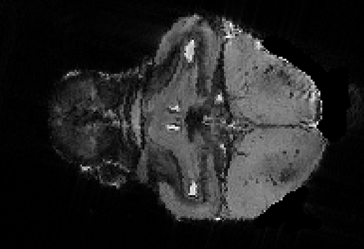
Here is what my window looks like after I right-clicked on the transverse view of the brain. In this case the minimum intensity I selected was too high, there are large parts of brain that are not labelled (i.e. not red) within the circle. The part of the brain outside the circle (the grey upper half of the transverse view) is not a problem.
I’ll try a lower minimum, 500. I press “Y” to open the threshold window, enter “500 33000” and click “Ok”. Then I go back to my three-views window and right click again in the same area. This is what I see:

I can see that the minimum threshold I’ve selected is too low. Area that is not brain, but is around the brain, has been included in my segment (the red area). I need to select a minimum threshold somewhere between 500 and 5000.
Next, I make sure my cursor is hovered over the transverse view (this tells Display that I want the action I’m about to take to apply to the transverse view and not either of the other two views) and I press “S” and then “B” to erase the segment I just made, and then the space bar to return to the segmentation menu.
Now I’ll try a minimum threshold in between the two I’ve already tried, 2000. Again, I press “Y”, then enter my threshold values “2000 33000”, then press “Ok”. Finally, I right click once again in the same part of the brain in the 3-views window. It looks like this:

This looks great! The edge of the red seems to match up well with the edge of the brain.
Now I want to fill in the rest of the brain. To do this I use the “Fill 3D” segmenting function. Hover the cursor over any part of the brain that is not segmented and press 6 on the keyboard. It doesn’t matter which of the three views of the brain the cursor is hovered over, but it must be hovered over unsegmented brain, i.e. it must be hovered over a part of the image that is grey or white, not red or black. The 3D Fill function takes a while to run on a normal computer, so give it a few minutes. When it’s done, it will say “done” in the Terminal and the 3-views window will look like this:

I cannot see any grey or white, all the parts of the image that are brain are red, indicating that the entire brain (except see next paragraph) is now segmented. The next step is to save the segment (aka label). To do this, press the space bar to go back to the main menu, then “T” to go to the file menu then “W” to save the label as a minc (.mnc) file. Pressing “W” will open up a save window that is identical to any other save window for any program, so navigate to the folder you want to save in, enter a file name, and click “save”. I recommend saving label files in the same folder as where the MRI image is located.
As I hinted at above, the entire brain has not actually been labelled. In a zoomed in sagittal view there are some “holes” visible in the segment of the brain:

These holes are places in the brain where the intensity is so low it becomes indistinguishable (by intensity) from empty space. These brain regions cannot be segmented by intensity. To fill in these regions, I use the dilation and erosion functions of the minc toolkit. Dilation and erosion can also be done in Display, but I prefer command line. Here is the command that does this:
$ mincmorph -successive DDDDDDDEEEEEEE CdecresiiModel.label.threshold.mnc CdecresiiModel.label.threshold.mincmorph.mnc
This command dilates (i.e. expands) the label seven times (each “D” is one dilation) and then erodes the label seven times. The successive dilations expand not only the outer edges of the label, but also all the inner edges (the holes) as well. With enough dilations, the holes are completely filled in. Each erosion then shrinks the label, however if a hole has been completely filled in by the dilations there is no edge there for the erosion to shrink from, so the hole stays filled in. More dilations fill in larger holes, and the number of dilations needed to fill in any particular set of holes is just trial and error. The number of erosions should be equal to the number of dilations or else the outer edge of the label will no longer match the outer edge of the brain. Too few erosions and the label will be larger than the brain, too many and it will be smaller.
I open the new label and the MRI image in Display using this command:
$ Display CdecresiiModel.mnc -label CdecresiiModel.label.threshold.mincmorph.mnc

Most of the holes are gone, but one large hole remains. I could go back and try a larger number of dilations to get rid of this hole, but since there is only one hole, it looks like it will take many dilations to get rid of it, and each dilation takes a while for my computer to run, I think I’ll just fill this hole using 3D segmentation. I can only do this because the hole is surrounded on all sides, in all three dimensions, by label. If it were on the edge of the brain, and continuous with the not brain, I would have to use manual segmentation to fill the hole. As it is, though, I am lucky and all I need to do is hover my cursor over the hole and press “F” “6”.

Now that the hole is filled, the label is done! What I need to do now is make a surface of this label. I press space then “T” and “W” to save my label and then exit Display.
Now, a confession. I don’t know how to make a surface using the minc toolkit. However, it is easy to do in ITK-SNAP, so I’m going to export my label and do it there. ITK-SNAP cannot read minc files, so first I convert my minc file to a NIFTI file:
$ mnc2nii CdecresiiModel.label.threshold.mincmorph.threshold.mnc CdecresiiModel.label.threshold.mincmorph.threshold.nii
Next, in ITK-SNAP, open the brain model as the main image by going to File > Open Main Image and the label as the segmentation by going to Segmentation > Open Segmentation. Then go to Segmentation > Export as Surface Mesh and save the surface. Finished!

The surface mesh (.stl) of the lizard brain.
Outstanding questions:
While going through this process I came across some questions that I wasn’t able to find the answers to. If you are reading this and familiar with the minc toolkit, I would very much appreciate it if you could contact me if you know the answers to these questions:
1) Is it possible to do intensity threshold-based segmentation from the command line in minc?
2) Can minc export surfaces in any of the following formats: STL, OBJ, PLY, FBX?
3) When I launch Display a 3D View window opens and then immediately closes. How can I keep this window and generate a 3D visualization of my label?